scatools

Introduction

We start by loading scatools and a filepath to an example fragments.bed.gz file containing fragments from 100 normal mammary cells.

Note this vignette is currently set up with dummy normal data and is purely intended to demonstrate package functionality. There are no CNV changes in the test data.

Installation

You can install the development version of scatools from GitHub with:

devtools::install_github("mjz1/scatools")

Example

We start by loading scatools, as well as the filepath to an example fragments.bed.gz file containing scATAC fragments from 100 normal mammary cells.

library(scatools)
library(dittoSeq)
library(ComplexHeatmap)
library(patchwork)

ncores <- 4 # Adjust accordingly

fragment_file <- system.file("extdata", "fragments.bed.gz", package = "scatools")

Now we process this data using scatools. Helper functions help us to create GenomicRanges bins, and compute GC content for downstream usage. Here we demonstrate using 10Mb bins.

Note: To generate your own bins object, a helper function is provided. Please note that running this function requires installation of a BSgenome of your choice. Here we use hg38.

# if (!require("BiocManager", quietly = TRUE))
# install.packages("BiocManager")

# BiocManager::install("BSgenome.Hsapiens.UCSC.hg38")

bins <- get_tiled_bins(
  bs_genome = BSgenome.Hsapiens.UCSC.hg38,
  tilewidth = 1e7,
  respect_chr_arms = TRUE
)

We load blacklist regions for our genome. These are used to remove fragments found in low mappability or high signal regions as defined here.

# Get blacklist regions
blacklist <- get_blacklist(genome = "hg38")

Then we run the pipeline:

sce <- run_scatools(
  sample_id = "test_sample",
  fragment_file = fragment_file,
  blacklist = blacklist,
  outdir = "./example/",
  verbose = TRUE,
  overwrite = TRUE,
  ncores = ncores,
  bins = bins
)

Plot the results using the dittoSeq package.

p1 <- dittoDimPlot(sce, var = "clusters")
p2 <- dittoDimPlot(sce, var = "tumor_cell")

p1 + p2 & theme(aspect.ratio = 1)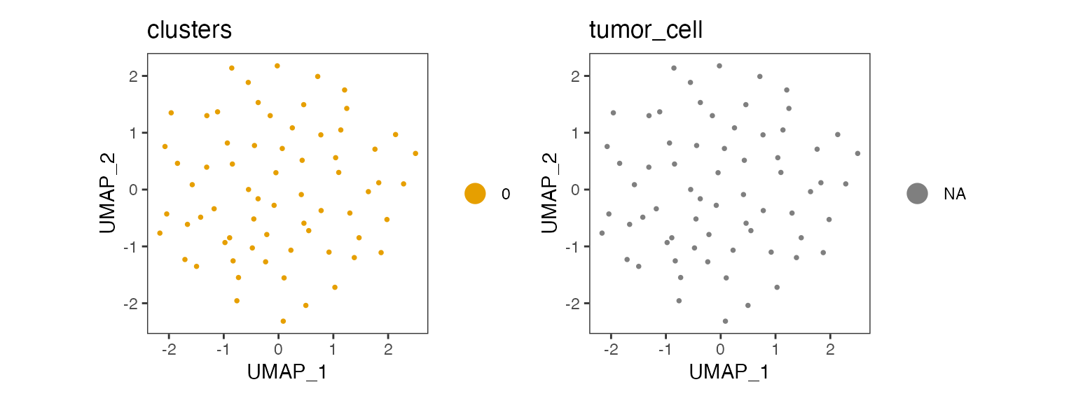

We can visualize the results as a heatmap.

sce <- sce[, order(sce$tumor_cell, sce$clusters)]

col_clones <- dittoColors()
col_clones <- col_clones[1:length(unique(sce[["clusters"]]))]
names(col_clones) <- levels(factor(sce[["clusters"]]))


left_annot <- ComplexHeatmap::HeatmapAnnotation(
  tumor_cell = sce[["tumor_cell"]],
  cnv_cluster = sce[["clusters"]],
  col = list(cnv_cluster = col_clones),
  which = "row"
)


p_ht_cna <- cnaHeatmap(sce, assay_name = "segment_merged_logratios", clust_annot = left_annot, col_fun = logr_col_fun())
p_ht_cna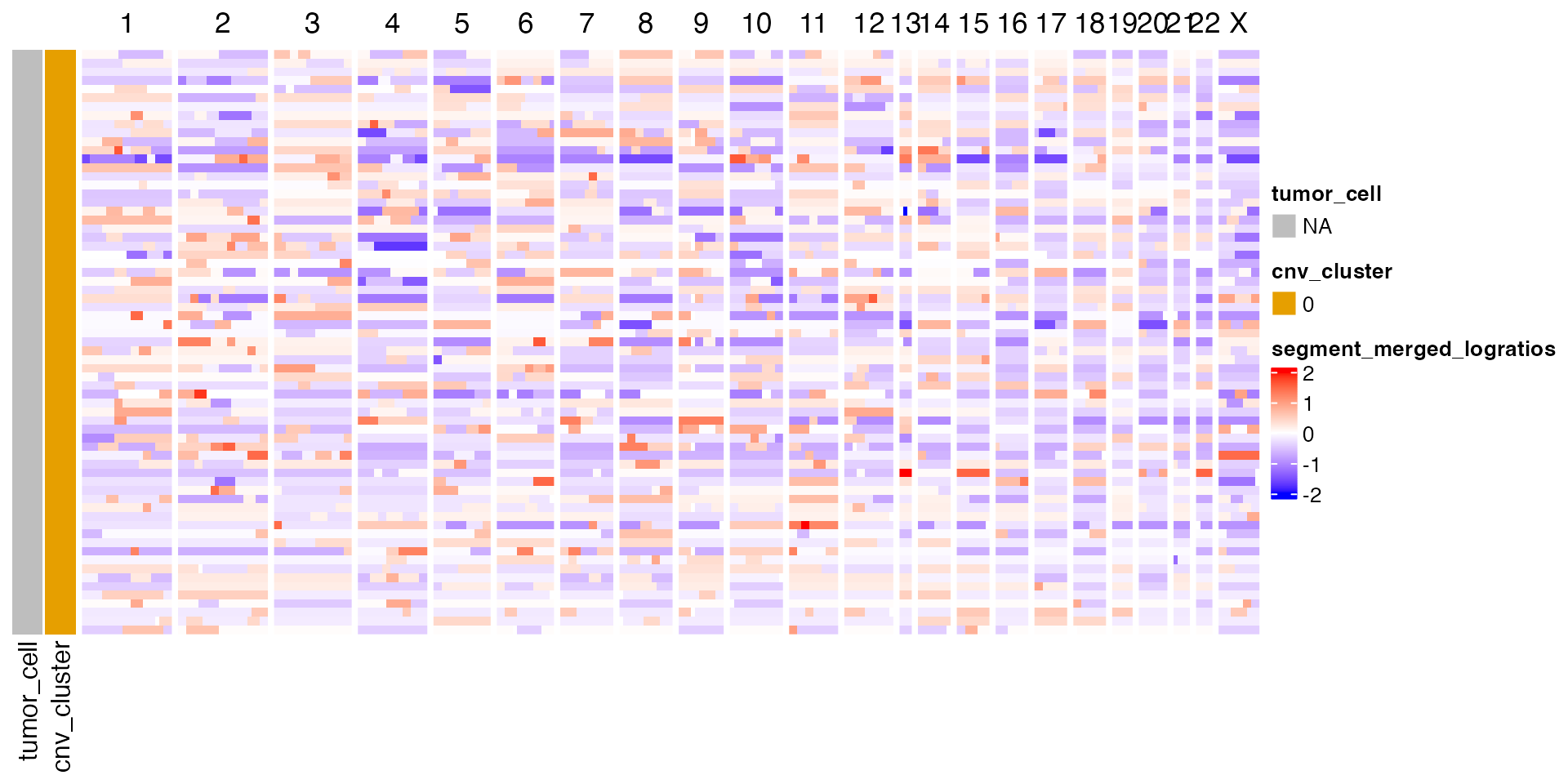

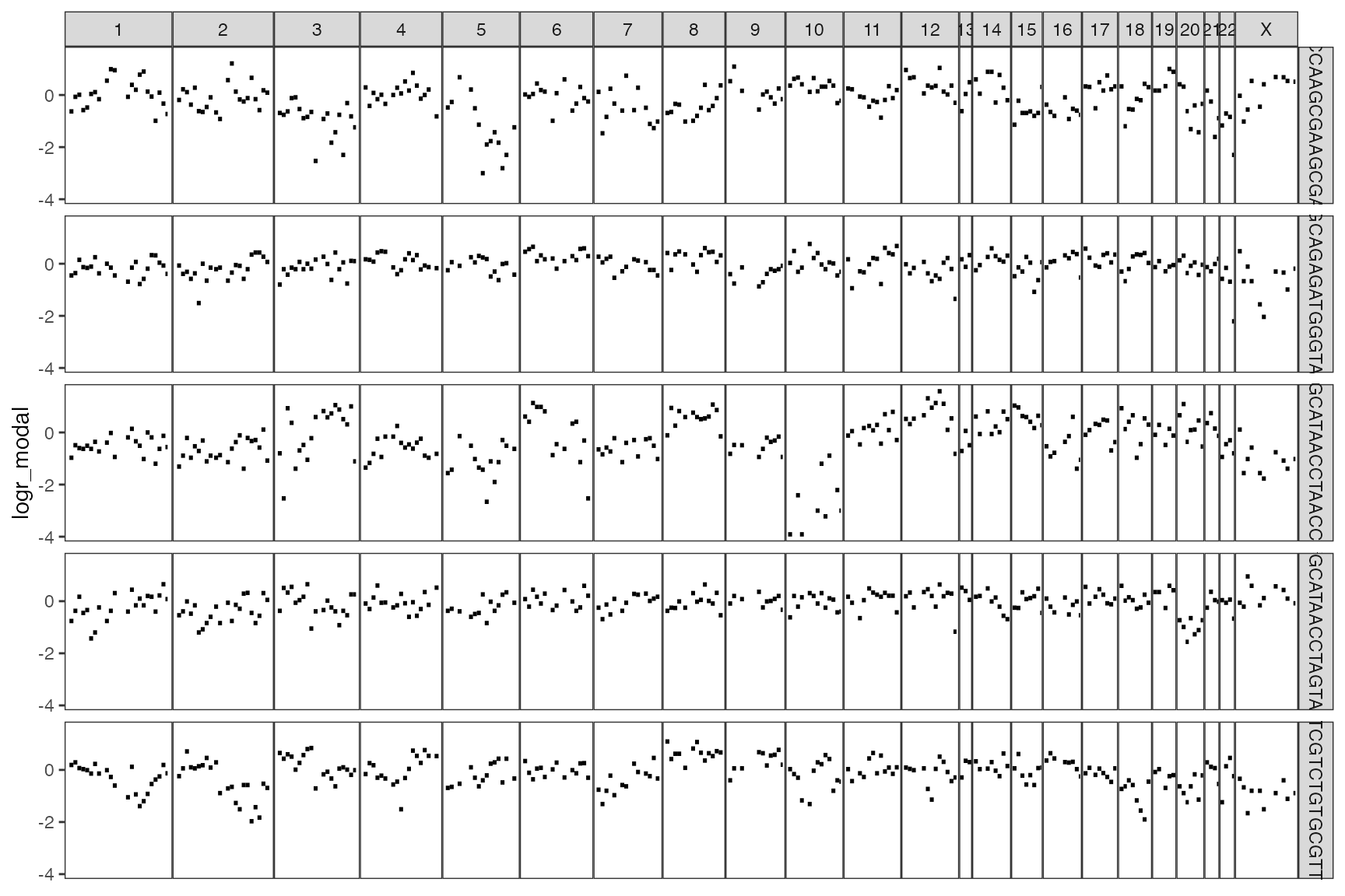
Or plot individual cells

# Plot the first five cells
plot_cell_cna(sce = sce, cell_id = 1:5, assay_name = "logr_modal")